A Simple
Circuit Implementation
of a Chaotic Lorenz System
Ned J. Corron
The Lorenz system is one of a few standard oscillators commonly used to explore chaos [1]. An accessible description of its mathematical features and chaotic dynamics is presented by Thompson and Stewart [2]. This important system was originally developed as a simplified mathematical model of atmospheric instabilities and does not derive from a basic circuit topology. As such, realizing an electronic Lorenz oscillator requires an explicit analog computer implementation of the oscillator equations. A few designs for realizing a Lorenz attractor have been published in the literature [3‑14]. Here, we present an original circuit design that is derived directly from the Lorenz system equations.
The Lorenz system is defined by the system of ordinary differential equations
 (1)
(1)
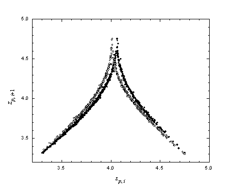
where X, Y, and Z are the states of the system and s, R, and b are parameters. Typical parameter values that yields chaotic dynamics are s = 10, R = 30, and b = 8/3. For these values, the attractor generated by numerically integrating (1) is shown in Figure 1. Typical waveforms for the three dynamical states are shown in Figure 2.

Figure 1. Lorenz attractor generated by numerical integration of the system equations with s = 10, R = 30, and b = 8/3.

Figure 2. Typical Lorenz waveforms generated by numerical integration of the system equations with s = 10, R = 30, and b = 8/3.
To obtain a practical circuit design for the Lorenz system, it is necessary to scale the system equations. To this end, we define the new system states
![]() (2)
(2)
where a is a scale parameter to be chosen. With the scaling (2), the system dynamics are governed by
 (3)
(3)
For a practical circuit, it is desirable to use ±10‑V signals to represent the system states. Based on the magnitude of the oscillations shown in Figure 1, choosing a = 1/3 yields states that map directly to the desired voltage range. As such, the scaled system is
 (4)
(4)
where x, y, and z are measured in volts. The Lorenz attractor for the scaled system (4) is shown in Figure 3.

Figure 3. Numerical Lorenz attractor for the scaled system with a = 1/3.
A circuit schematic that closely realizes the scaled Lorenz system is shown in Figure 4. The voltages at the nodes labeled x, y, and z correspond to the states of the scaled system (4). The multipliers are each AD633, for which the additional summing node is grounded. The operational amplifiers are all TL082 or equivalent. The circuit is powered with ±15 V. Since the input to the AD633 is very high impedance, the three-volt reference for Va can be implemented using resistors as a voltage divider; however, it is preferable to use a Zener diode or other fixed voltage reference to make the circuit independent to changes in the supply voltages. As drawn, the circuit oscillates near 2 kHz; however, to vary the frequency without affecting the chaotic nature, all three capacitors may be scaled equally.
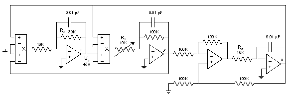
Figure 4. Lorenz circuit schematic.
The oscillator parameters R, s, and b for the Lorenz circuit are controlled with three circuit resistors. The R parameter is set with the variable resistor RR by the relation
![]() (5)
(5)
Similarly, the s and b parameters are set by the resistors Rs and Rb via
![]() (6)
(6)
and
![]() . (7)
. (7)
Often for bifurcation studies of the Lorenz system dynamics, the parameter R is varied while s and b are held fixed; as such, RR is implemented here using a variable resistor. Clearly, variable resistors can also be used for Rs and Rb if one desires to adjust these parameters while the circuit is running. The scale parameter a is set with the reference voltage Va using
![]() (8)
(8)
where Va is measured in volts.
As drawn in Figure 4, the circuit is configured for s = 10, b = 8/3, a = 1/3, and a variable R. Using a 10 kW potentiometer for RR yields the range 3 ≤ R < ∞, and setting RR ~ 1 kW provides a chaotic output with R ~ 30. An attractor measured from the circuit with these parameters is shown in Figure 5. Corresponding typical captured waveforms are shown in Figure 6.

Figure 5. Lorenz attractor measured from circuit.

Figure 6. Typical waveforms measured from Lorenz circuit.
It is
important to note that the Lorenz system equations are symmetric under the
transformation ![]() . Technically, this symmetry makes the system structurally
unstable. That is, arbitrarily small deviations in the mathematical description
of the oscillator will destroy this symmetry and result in a qualitatively
different system. In terms of a physical circuit, this is bad news, since an
exact realization of the equations is impossible due to limited precision of
the circuit components. As a result, a Lorenz circuit will exhibit asymmetric
oscillations, although the degree of asymmetry can be minimized using
high-precision components and trimmers. Unfortunately, the effects of the
asymmetry can be significant in circuits with analog multipliers, which are
notable for output voltage offset errors. Such errors, if uncompensated, can
lead to a obvious imbalance in the attractor exhibited by the circuit.
. Technically, this symmetry makes the system structurally
unstable. That is, arbitrarily small deviations in the mathematical description
of the oscillator will destroy this symmetry and result in a qualitatively
different system. In terms of a physical circuit, this is bad news, since an
exact realization of the equations is impossible due to limited precision of
the circuit components. As a result, a Lorenz circuit will exhibit asymmetric
oscillations, although the degree of asymmetry can be minimized using
high-precision components and trimmers. Unfortunately, the effects of the
asymmetry can be significant in circuits with analog multipliers, which are
notable for output voltage offset errors. Such errors, if uncompensated, can
lead to a obvious imbalance in the attractor exhibited by the circuit.
To
illustrate the asymmetry in a practical implementation, we consider the peak
return map on the strictly positive state z. In Figure 7, a return map for successive
maxima in the z state obtained from a
numerical integration of the Lorenz system equations is plotted. As evident in
this figure, the dynamics of the Lorenz system is well modeled by a unimodal, one-dimensional return map [15]. Such a simplification is
important, especially in the application of symbolic dynamics to this system [16]. In particular, it is known
that a generating partition exists at the maximum in such a return map, and
that an infinite sequence of returns above and below this partition (i.e., symbols 1 and 0, respectively) uniquely
defines a trajectory for the iterated system. However, for the Lorenz system,
there is an ambiguity in the sign of the states x and y due to
the symmetry inherent in the system equations. With each return above the
partition (i.e., with each symbol 1),
the state of the system switches across the symmetry, flipping the sign of the x
and y states; however, determining the absolute state of the system with
respect to this symmetry requires knowing the sign of the initial state of the
system.

Figure 7. Peak return map on z from numerical integration of the Lorenz system equations.
In Figure 8, we show the peak return map measured for an actual Lorenz circuit. Here, it is apparent that the return map is more complex and the dynamics of the circuit are not well defined by a simple one-dimensional return map. This complication is due to the inevitable loss of symmetry due to a physical implementation. To illustrate the asymmetry, peak returns with positive x and y are shown as open circles in the figure, while those with negative x and y are shown filled. It is evident that the loss of symmetry has resulted in twin maps, offset by roughly 0.05 V, corresponding to returns on each side of the attractor. Trimming the offsets of the two analog multipliers in the circuit could be used to reduce this asymmetry, but true symmetry is impossible to achieve in any physical system.
In conclusion, we have shown a simple circuit implementation of the chaotic Lorenz system. This oscillator circuit is capable of producing the interesting nonlinear dynamics of this important system, including chaos. Besides obvious pedagogical applications, this circuit may be also well suited for technological applications, including communications via controlled symbolic dynamics [16]. However, it is important to realize that the idealized symmetry of Lorenz’s original mathematical model cannot be perfectly achieved in any physical realization, and any experiments designed to use this circuit must not hinge critically upon realizing perfect symmetry.
References
1. E. N. Lorenz, “Deterministic nonperiodic flow,” J. Atmos. Sci. 20(2), 130-141 (1963).
2. J. M. T. Thompson and H. B. Stewart, Nonlinear Dynamics and Chaos (Wiley, New York, 1986).
3. R. Tokunaga, M. Komuro, T. Matsumoto, and L. O. Chua, “‘Lorenz attractor’ from an electrical circuit with uncoupled continuous piecewise linear resistor,” Int. J. Circ. Theory Appl. 17(1), 71-85 (1989).
4. K. M. Cuomo and A. V. Oppenheim, “Chaotic signals and systems for communications,” Proc. IEEE ICASSP, vol. 3, 137-140 (1993).
5. K. M. Cuomo and A. V. Oppenheim, “Circuit implementation of synchronized chaos with applications to communications,” Phys. Rev Lett., 71(1), 65-68 (1993).
7. E. Sánchez and M. A. Matías, “Experimental observation of a periodic rotating wave in rings of unidirectionally coupled analog Lorenz oscillators,” Phys. Rev. E 57(5), 6184-6186 (1998).
8. O. A. Gonzales, “Lorenz-based chaotic cryptosystem: a monolithic implementation,” IEEE Trans. Circuits Syst. I 47(8), 1243-1247 (2000).
9. S.-C. Tsay, C.-K. Huang, D.-L. Qiu, and W.-T. Chen, “Implementation of bidirectional chaotic communication systems based on Lorenz circuits,” Chaos, Solitons, and Fractals 20(3), 567-579 (2004).
10. R. Nunez, “Comunicador experimental privado basado en encriptamiento caótico,” Revista Mexicana De Fisica 52(3), 285-294 (2006).
11. R. Nunez, “Encriptador experimental retroalimentado de Lorenz con parámetros desiguales,” Revista Mexicana De Fisica 52(4), 372-378 (2006).
12. E. Sánchez, D. Pazó, and M. A. Matias, “Experimental study of the transitions between synchronous chaos and a periodic rotating wave,” Chaos 16(3), 033122 (2006).
13. Jonathan N. Blakely, Michael B. Eskridge, and Ned J. Corron, "A simple Lorenz circuit and its radio frequency implementation," Chaos 17(2), 023112 (2007).
14. Jonathan N. Blakely, Michael B. Eskridge, and Ned J. Corron, “High-frequency chaotic Lorenz circuit,” Proc. IEEE SoutheastCon 2008, 69-74 (2008).
15. P. Collet and J. P. Eckmann, Iterated Maps of the Interval as Dynamical Systems (Birkhauser, Boston, 1980).
16. E. M. Bollt, “Review of chaos communication by feedback control of symbolic dynamics,” Int. J. Bifur. Chaos 13(2), 269-285 (2003).

